On this page Brute forcing it
I wanted to learn auto-routing for photonic chips. The story below is how I got there: a failed brute-force attempt, then using AI as a learning partner, then building interactive HTML routing arenas, then translating that into a PhotonForge router, and finally wrapping an auto-design agent around the whole thing.
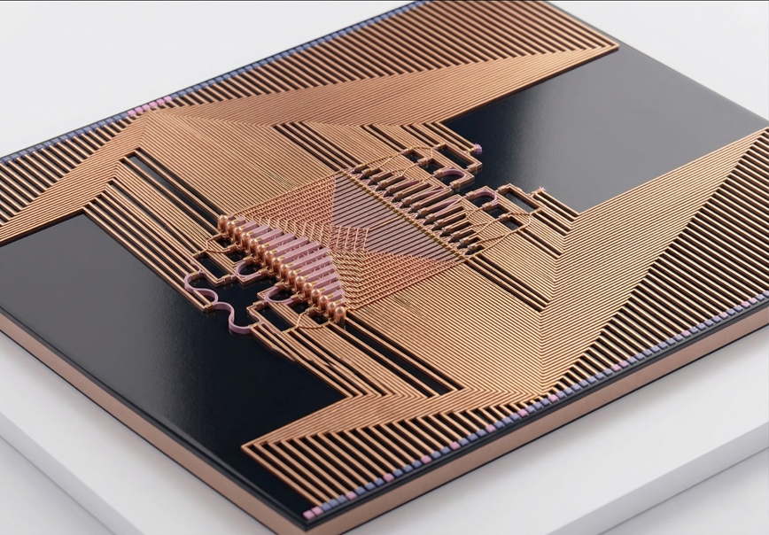
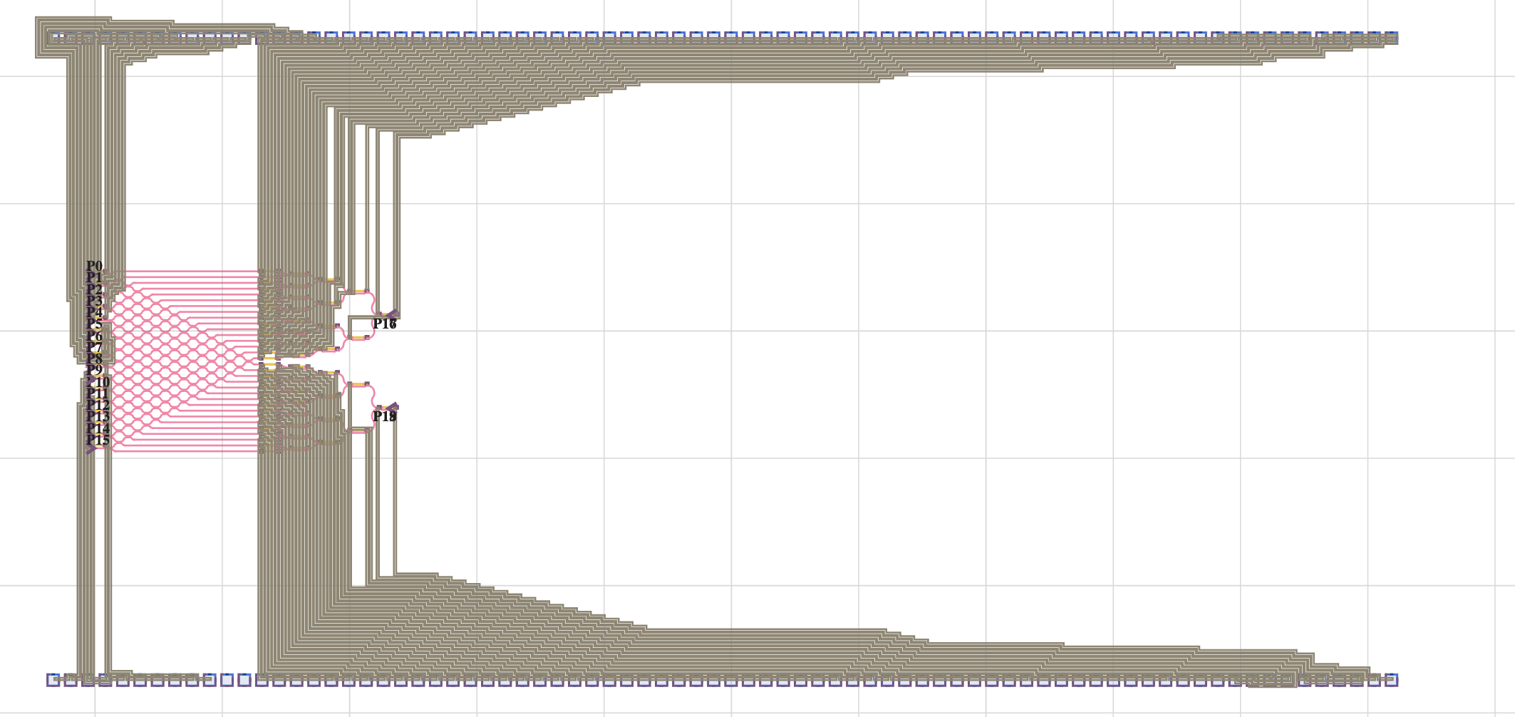
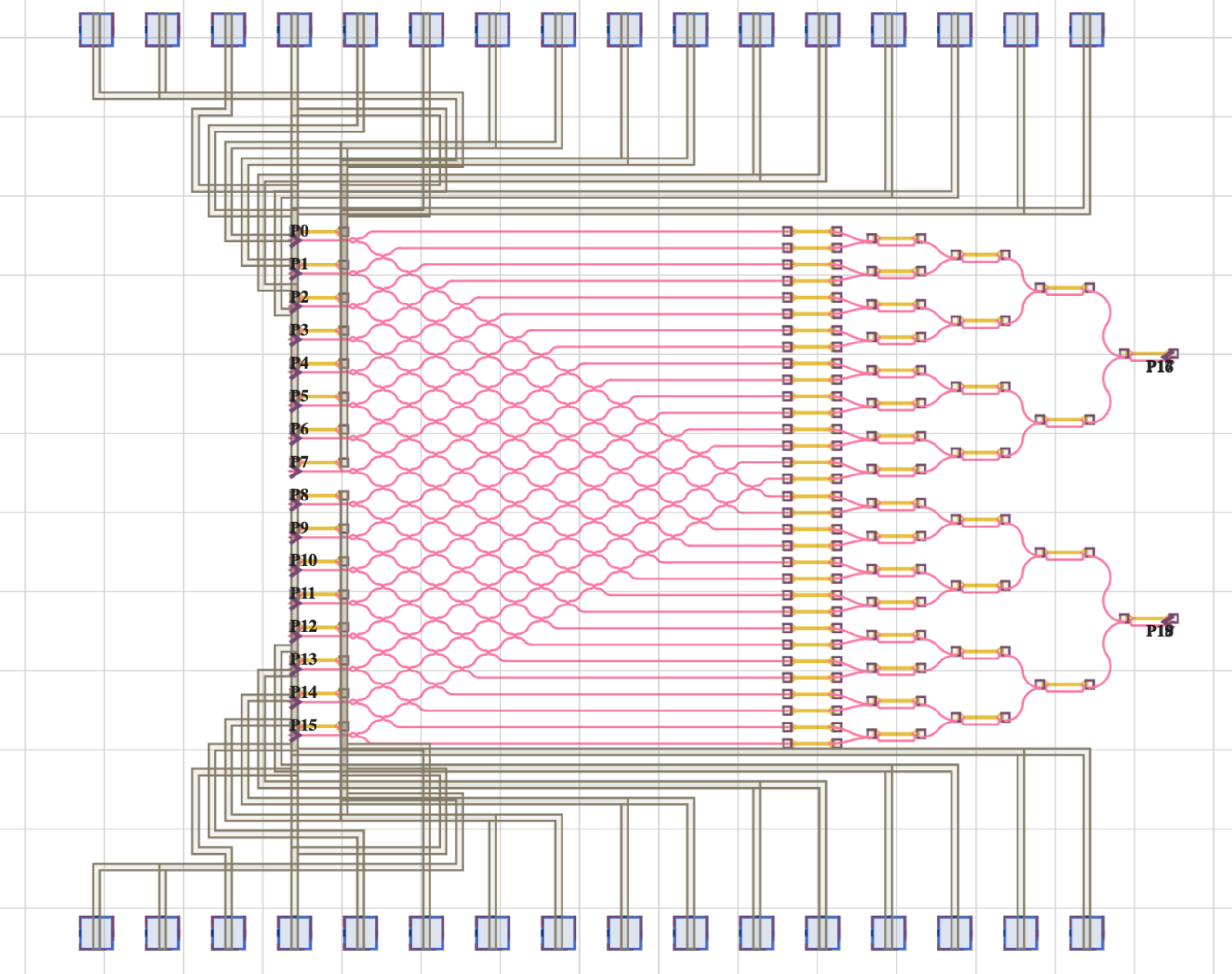
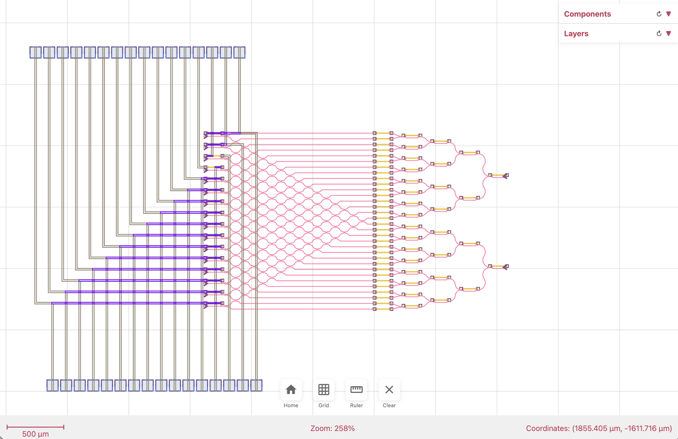
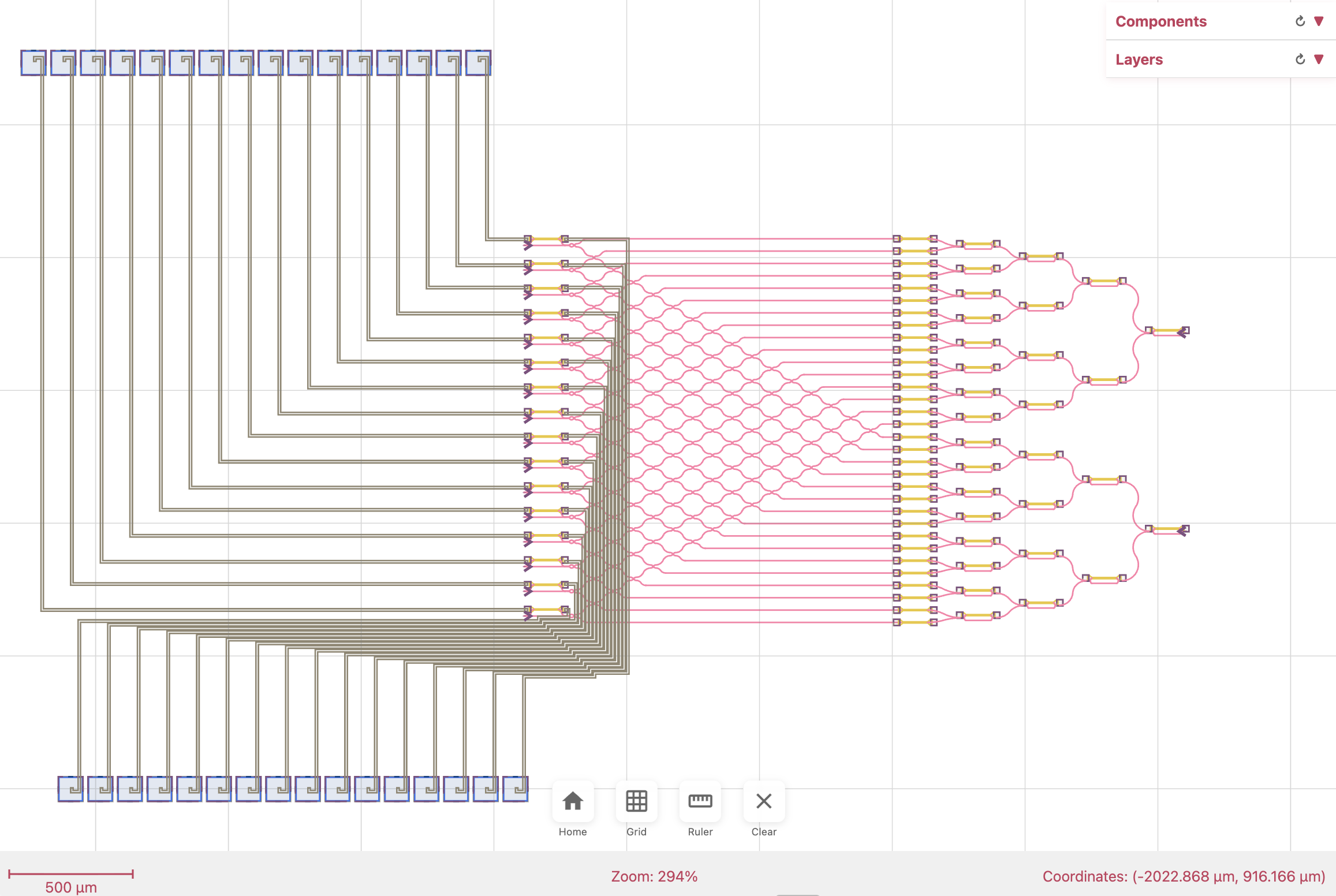
The kind of chip we end up routing: dozens of active elements, each needing a trace to a bondpad.
Brute forcing it
My first instinct was lazy and honest. I opened Claude Code, dropped in screenshots of a half-routed projector chip, and asked the model to fix the layout by editing PhotonForge’s route_manhattan call. No algorithm in mind, no plan, just “make this work.”
It sort of worked. And then it didn’t.
Second attempt after several rounds of tweaks: cleaner, but still hand-waved and fragile.
Each round of “please fix this” traded one failure for another. Waypoints helped two nets and broke three. A tweak that untangled the left half pushed the mess to the right half. The AI was writing plausible code, and I was nodding along, but neither of us actually understood routing. We were patching symptoms.
This is the trap that’s easy to miss: AI is so good at producing code that reads right that you can spend days iterating without stepping back to ask the real question.
Using AI as a learning partner
So I stopped asking for code and started asking for a map of the territory. What does this problem look like when people have thought about it carefully?
The AI pointed me at a 60-year-old field: VLSI and PCB autorouting. Lee’s algorithm from 1961, A* with Manhattan heuristics, Dijkstra over weighted cost fields, PathFinder-style negotiation routing, rip-up and reroute from commercial EDA tools. And then it pointed me at the best single resource it knew of: Rob Rutenbar’s VLSI CAD: Logic to Layout lecture series from the University of Illinois, weeks 7 and 8 specifically, free on the Internet Archive.
I watched them. Not skimmed, watched. And this is where the story changes. From this point on, the AI is no longer guessing with me. It is helping me build and test ideas I actually understand.
Building an HTML routing arena
Routing is spatial. Reading about BFS wavefront expansion does not click until you see the wavefront propagate across a grid. So I asked the AI to build me interactive visualizers. Not in Python, not in a Jupyter notebook, in pure HTML with Canvas, so I could open them on my phone, on the couch, with zero setup.
Each lecture concept turned into an interactive prototype within minutes. Click to place a source, a target, and obstacles. Step through BFS one layer at a time. Watch the wavefront wrap around walls. Trace the shortest path back. Then: add a second net, then four, then a cost-field heatmap for bundling.
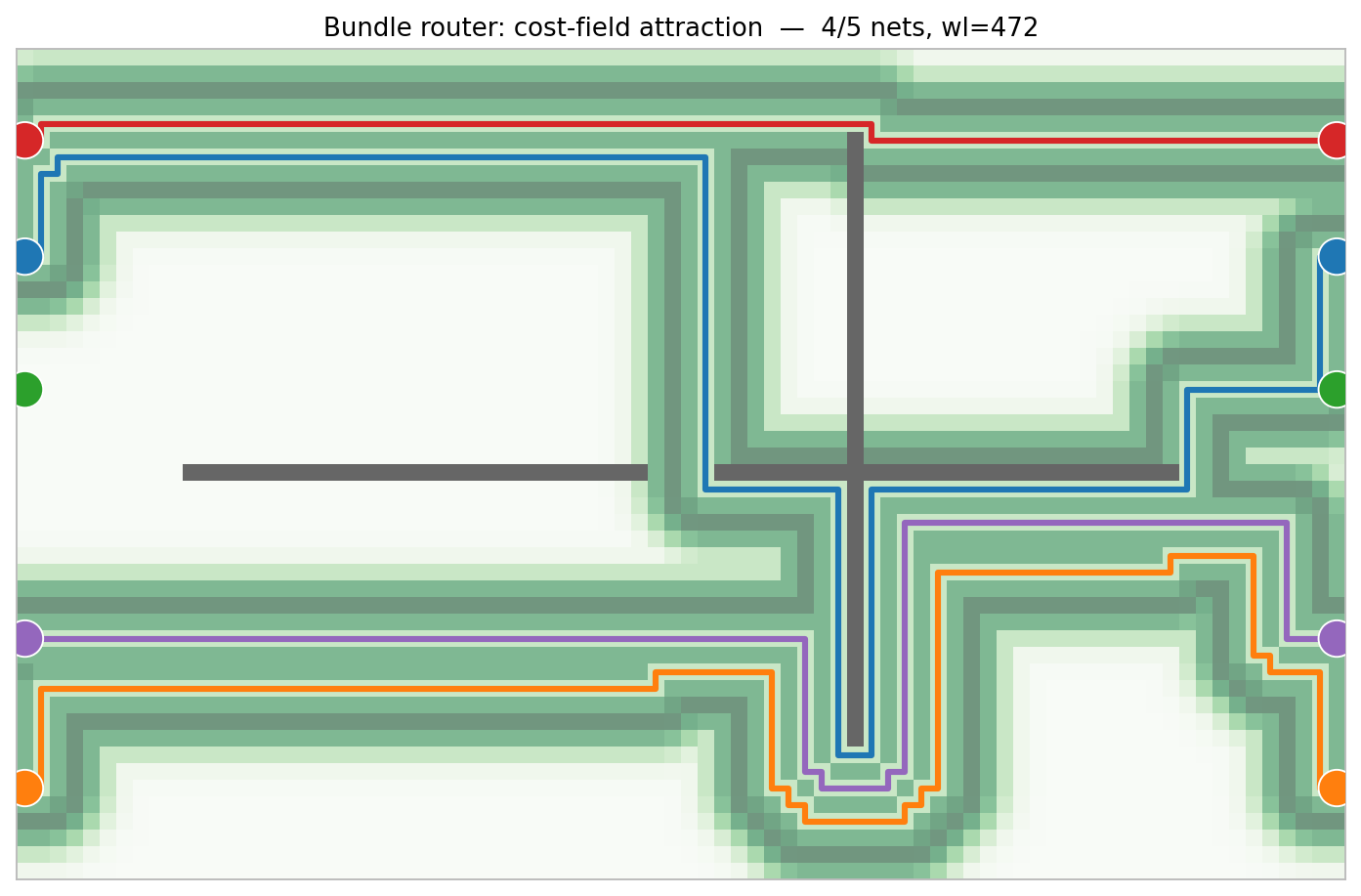
Bundle router with its cost-field overlay. Existing routes emit a soft attraction field; new routes settle into the channel one cell away. Making the field visible made the algorithm obvious.
Once the building blocks worked, I stacked them into a comparison arena that runs twelve algorithms on the same obstacle layout and the same nets, side by side.
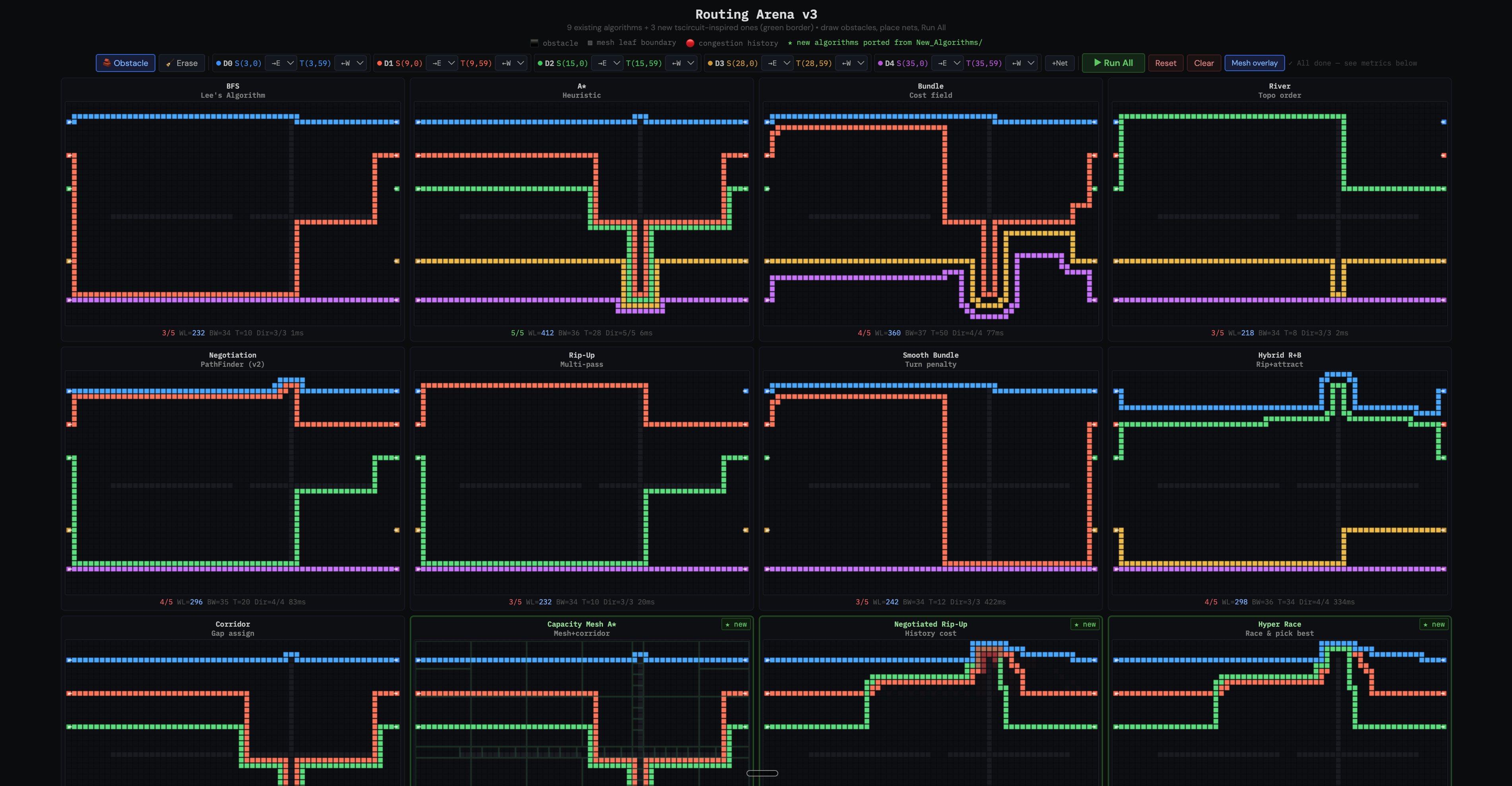
Twelve algorithms on one 5-net problem. Each has a different personality. A* and Corridor complete all 5 nets but route wide. Rip-Up and Hybrid route shortest but leave some nets for later. Bundle and Smooth Bundle hug existing routes. River fails topologically.
The arena made trade-offs visceral. I could drag obstacle walls around with a slider and watch every algorithm respond in real time. New hybrid strategies (rip-up plus bundle, smooth bundle with turn-cost penalties) came out of playing with the arena, not from staring at pseudocode.
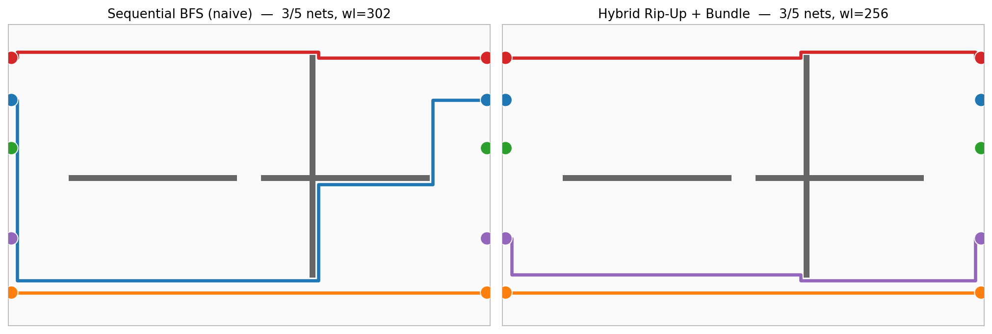
The two ends of the spectrum on the same problem: naive Sequential BFS (left) and Hybrid Rip-Up
- Bundle (right). Same nets, same obstacles, very different cost and topology.
Why HTML was the right medium
I want to single this out because it felt counterintuitive at first. The algorithms themselves are Python-native, and the production target is PhotonForge. Why prototype in a browser?
Because the point of the prototype was to build my intuition, not to ship code. HTML means zero setup, works on any device, and Canvas makes it trivial to animate the wavefront at a rate a human can follow. Every time I wanted to understand something — why does net ordering matter? what does the congestion history look like after iteration 5? what turn-penalty kills the sawtooth pattern? — I could have an interactive answer in minutes. That loop is what learning looked like.
Translating to a PhotonForge router
Once the algorithms were intuitive on an abstract grid, translating them to PhotonForge was mechanical. The architecture has two layers:
- Algorithm layer: pure Python on an integer grid. Takes source and target cells, avoids obstacle cells, returns a list of grid coordinates. No dependency on PhotonForge.
- Integration layer: a thin bridge that converts PhotonForge layout coordinates to grid cells, rasterizes structures on a given metal layer into obstacles, runs the algorithm, and converts the result back into a
Pathon the routing layer.
from pf_routing_arena import PFRoutingArena
from routing_algorithms import HybridRipUpBundle

arena = PFRoutingArena(
    bbox_min=(-200, -200), bbox_max=(2200, 1400),
    grid_pitch=25, router_class=HybridRipUpBundle,
)
arena.add_obstacles_from_layer(component, M2_layer, margin=1)
arena.add_obstacles_from_layer(component, M1_heater, margin=1)

for i in range(n_nets):
    arena.add_terminal_pair(f'D{i}', left[i]['T0'], right[i]['T0'],
                            source_dir='E', target_dir='W')

results = arena.route_all(trace_width=20, layer=M2_layer)
The integration work was almost entirely about the boundary between the grid world and the layout world: reserving a net’s own pad exit zone while keeping other pads blocked, rasterizing heater pads on a different metal layer as routing obstacles, and enforcing a 1-cell margin between committed routes so they do not physically overlap at real trace widths.
I prototyped all of this in a Jupyter notebook first, then moved it to the library. The notebook let me flip between algorithms on the same layout and see the difference, which is the same feedback loop the HTML arena gave me, just now in the domain that ships.
Scaling up: the auto-design agent
This is where I thought I was done. Twelve algorithms, a clean bridge to PhotonForge, a notebook that can route a small test layout. Ship it.
Then I pointed it at a real quantum photonic chip with 32 active elements, each needing a metal trace to its own bondpad, with heaters and other obstacles scattered through the middle. Picking an algorithm was no longer the hard part. The hard parts were all the human decisions an engineer makes before the router ever runs: how to pair pins with bondpads, where to place the bondpad row, what directions to let routes approach from, how wide the trace should be.
No single algorithm solves those. They are design decisions, and they interact. Change the bondpad row position and the net-to-pad assignment flips. Change the assignment and the approach directions become wrong. Change the trace width and obstacle inflation changes with it.
This is the regime where an auto-design agent earns its keep. You give it a goal, the tools to build a layout, a design-rule checker that counts violations, and let it propose, try, measure, and revise.
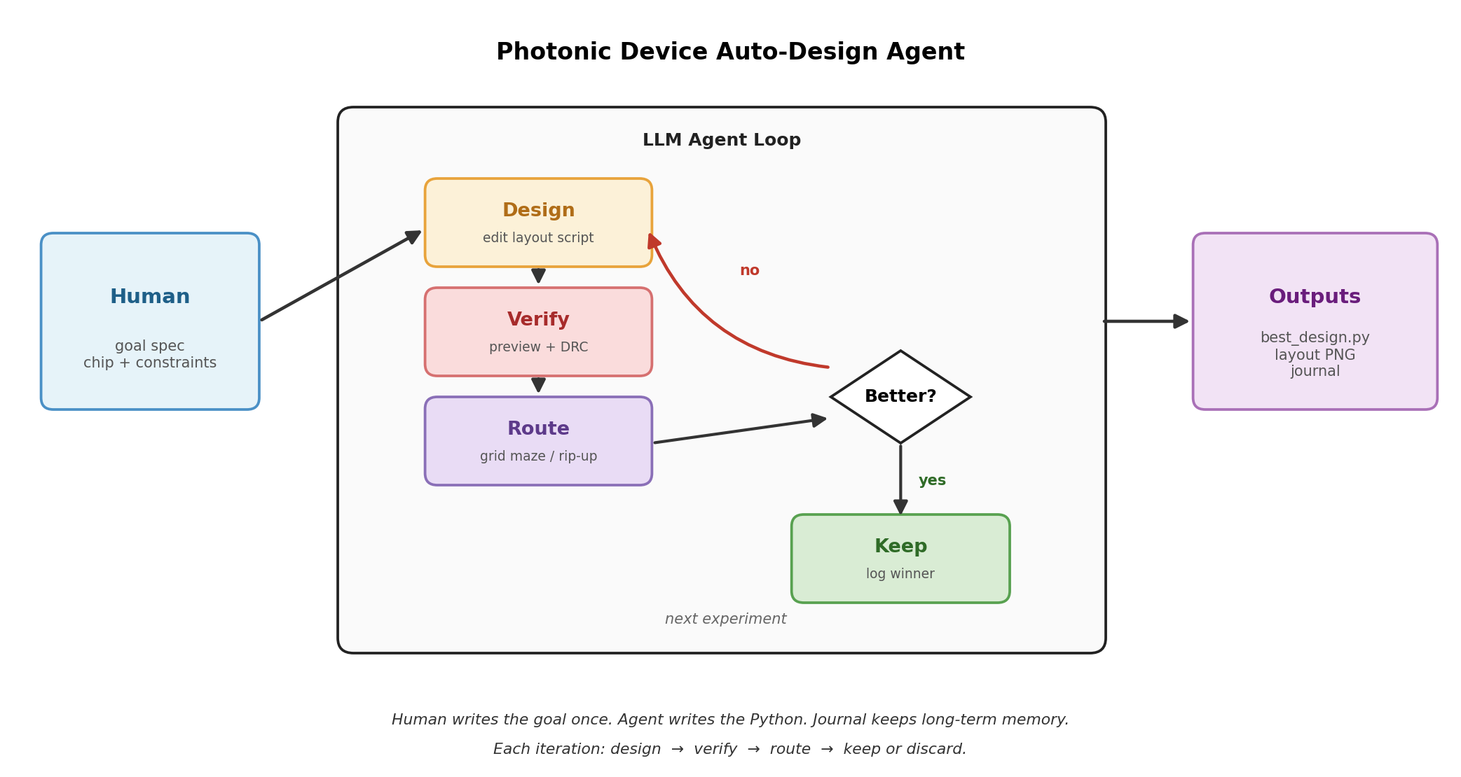
The Auto-Design loop. A human writes the goal once. The agent edits the routing script, PhotonForge builds the layout, the DRC returns pass or fail counts, and a journal remembers every attempt.
The baseline was bad on purpose
The starting script was the laziest possible: call route_manhattan independently for each of 32 pin-to-pad connections and hope.
That first attempt produced 192 violations: 30 heater crossings and 162 pairs of routes crossing each other.
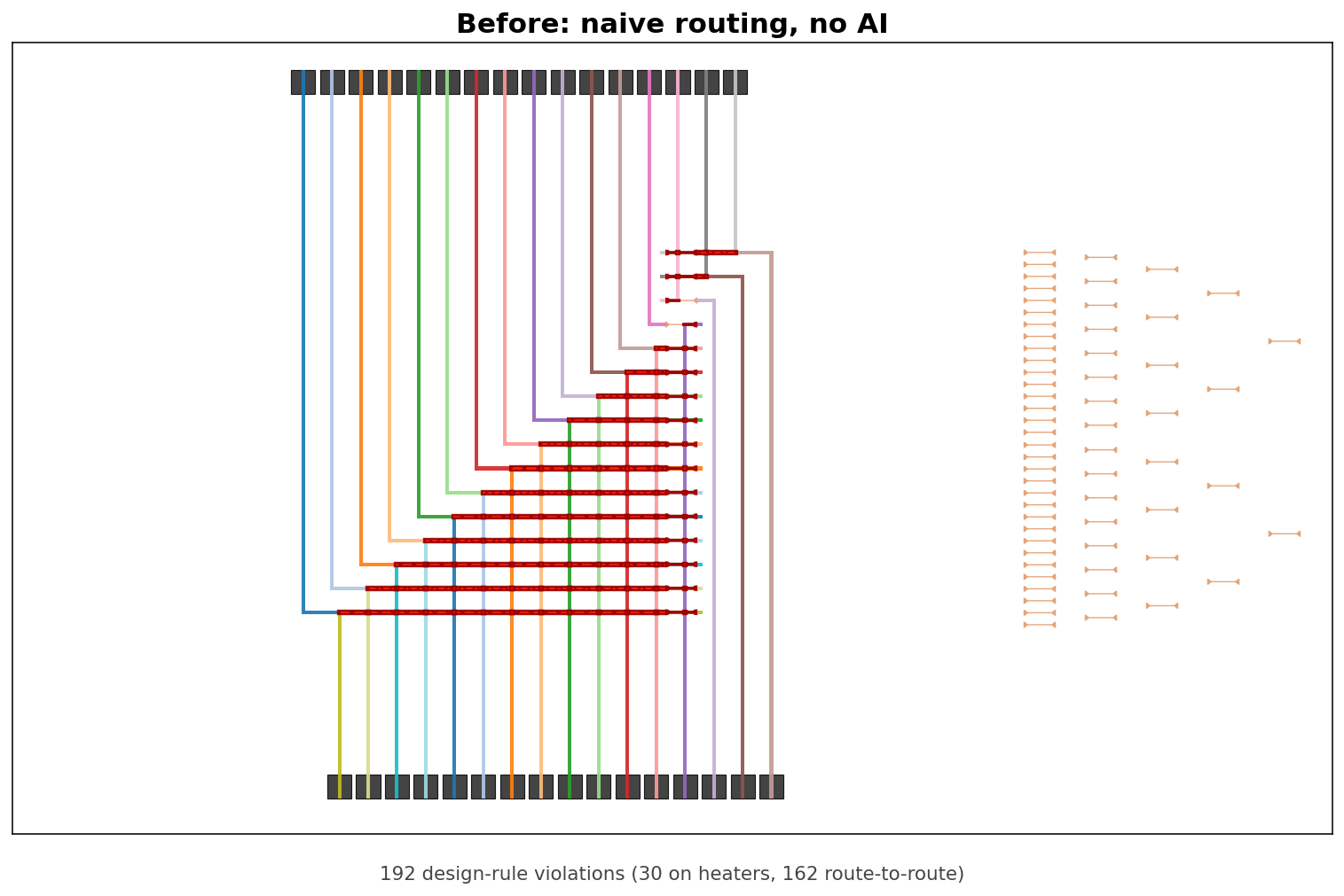
The starting point in PhotonForge. Every net routes selfishly and hits everything else.
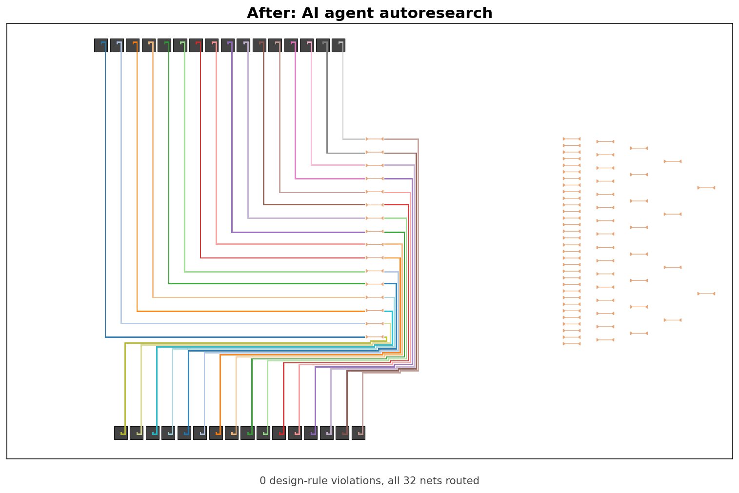
What the agent did
Over 27 iterations the agent:
- Switched from independent Manhattan routing to a grid-based planner so nets could share the chip.
- Taught the planner to treat heaters as obstacles, not just metal layers.
- Swept polygon inflation (2, 5, 8.5, 12 µm) to find the right trace-to-obstacle margin.
- Tried four pin-to-bondpad assignment strategies (split by AMZI, split by terminal, x-sort, nearest).
- Shifted the bondpad row farther from the active area and swept its spacing.
- Diagnosed a last-mile edge case where one contact sat awkwardly close to a heater and fixed it with a single approach-direction constraint.
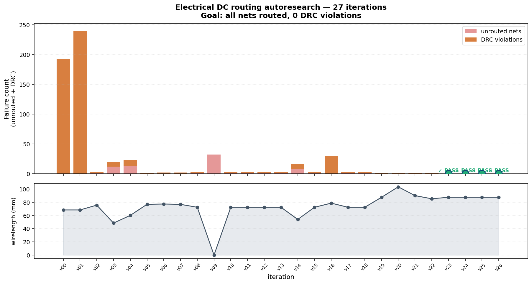
Violations and unrouted nets across 27 iterations. The four green circles mark the passing configurations.
Total wall-clock for all 27 iterations: 2 minutes 25 seconds. A human engineer laying this out by hand — pairing pins to pads, sketching the bundles, chasing the last DRC violations — typically needs two to three hours.
What I learned
The shortest version of this story: the AI did not replace the thinking, it compressed the distance between question and interactive answer.
The brute-force attempt failed because I was outsourcing the understanding. The learning partner approach worked because I stopped. The lectures still had to be watched. The wavefront still had to be visualized with my own eyes. The pin-reservation bug still had to be diagnosed by me, not narrated by the model.
But everything between “I want to explore this idea” and “I can see this idea running” collapsed. Interactive HTML prototype in minutes. PhotonForge bridge in an afternoon. Twelve algorithms ready to compare by the end of a weekend. And finally, an auto-design agent that picks up those algorithms and runs them 27 times in the time it takes to make coffee.
You can outsource implementation friction, algorithm discovery, and visualization scaffolding. You cannot outsource understanding. The surprise is that this style of working actually forces deeper understanding than the old way, because you are constantly building and testing your mental model instead of reading about someone else’s.
Interested in testing these algorithms on your own layout? Reach out to prash@flexcompute.com.